Code
using Plots, LaTeXStrings, Polynomials

function f₁( x )
    return x + rand()
end

function f₂( x )
    return 1/( 1 + exp( x ) );
end

function f₃( x, α = 25 )
    return 1/( 1 + α*x^2 );
end

f₄ = t -> max(0, @. 1-abs(t) );Lecture 6: Chapter 3: Polynomial interpolation
These lecture notes are mainly a record of what we discussed in class. They should not be used as a replacement for attending lectures or reading books. Please let me know if you find any errors or have any questions about the material.
You can use the Hypothesis commenting system available on the right side panel (you can login with your U/Google account). This allows you annotate the notes (private) and leave comments or reply to other people’s comments (public).
I encourage you to download the lecture notes and play around with the Julia code.
using Plots, LaTeXStrings, Polynomials
function f₁( x )
return x + rand()
end
function f₂( x )
return 1/( 1 + exp( x ) );
end
function f₃( x, α = 25 )
return 1/( 1 + α*x^2 );
end
f₄ = t -> max(0, @. 1-abs(t) );Interpolation Problem:
Suppose that \(X = \{ x_0 < \cdots < x_n \}\) is a set of distinct interpolation nodes, \(0 \leq m_0, \dots, m_n \leq m\), and \(f\) is an \(m\) times differentiable function.
Aim: find \(p\) such that
\[ \begin{align} p(x_j) &= f(x_j), \nonumber\\ % p'(x_j) &= f'(x_j), \nonumber\\ % &\vdots \nonumber\\ % p^{(m_j)}(x_j) &= f^{(m_j)}(x_j). \end{align} \tag{6.1}\]
for all \(j = 0, \dots, n\).
Example 6.1 (Taylor polynomial) If \(X = \{ x_0 \}\), then we can solve the interpolation problem with a polynomial of degree \(m_0\):
\[\begin{align} p(x) &= f(x_0) + f'(x_0)(x-x_0) + \cdots \nonumber\\ % &\qquad+ \frac{f^{(m_0)}(x_0)}{m_0!}(x-x_0)^{m_0} % \nonumber \end{align}\]
Exercise 6.1 Show that the degree \(m_0\) Taylor polynomial of \(f\) about \(x_0\) solves (6.1) when \(X = \{ x_0 \}\).
Definition 6.1 If \(X = \{ x_0 < \cdots < x_n \}\) and \(m_0 = m_1 = \cdots = m_n = 0\), we call (6.1) a Lagrange interpolation problem.
Theorem 6.1 (Lagrange interpolation) For \(x_0 < \cdots < x_n\) (nodes) and a function \(f\) defined on \(X = \{x_0,\dots,x_n\}\), there exists a unique polynomial interpolant \(I_Xf\) of degree at most \(n\) such that \(I_Xf(x_j) = f(x_j)\) for all \(j=0,\dots,n\).
In the following, we will write \(\mathcal P_n := \big\{p(x) = \sum_{j=0}^n a_j x^j \colon a_0, \dots,a_n \in \mathbb R\big\}\) for the set of polynomials of degree at most \(n\).
N = 10
X = range( -1, 1, N+1)
Y = f₁.(X)

scatter( X, Y,
    primary = false, markersize = 5 )
p = fit( X, Y )
plot( p ,
    xlims=(-1.05,1.05), legend = false, lw = 3)
scatter!( X, Y,
    primary = false, markersize = 5, color="green")
Proof. Existence: Use the Lagrange polynomials:
\[\begin{align} \ell_j(x) = \prod_{k\in\{0,\dots,n\}: \,\, k\not=j} \frac {x - x_k} {x_j - x_k} \end{align}\]
which satsisfy \(\ell_j \in \mathcal P_n\) and \(\ell_j(x_k) = \delta_{jk}\) for all \(j,k=0,\dots,n\).
Notice that
\[\begin{align} p(x) = \sum_{j=0}^n \ell_j(x) f(x_j) \end{align}\]
therefore satisfies \(p(x_k) = \sum_{j=0}^n \ell_j(x_k) f(x_j) = \sum_{j=0}^n \delta_{jk} f(x_j) = f(x_k)\) for each \(k=0,...,n\). That is \(p\) solves the Lagrange interpolation problem.
Uniqueness: suppose that \(q \in \mathcal P_n\) interpolates \(f\) at \(X\). Then, \(p - q\) has zeros at each \(x_j\), we have that \(x - x_j\) divides \(p-q\): that is \(p(x) - q(x) = \alpha (x - x_0)(x- x_1) \cdots (x - x_n)\). Since \(p-q\) only has degree at most \(n\), we must have \(\alpha=0\) and thus \(p = q\).
Here, we plot the Lagrange polynomials that appear in the above proof:
# X = @. cos( π*(0:N)/N )
X = range(-1,1,N+1)

function ℓ( j, x )
    r = 1;
    for n = 0:N
        if (n != j)
            r = r*(x - X[n+1]) / (X[j+1] - X[n+1])
        end
    end
    return r
end

anim = @animate for j ∈ 0:N
    p = x -> ℓ(j, x)
    plot(p, -1, 1,
        ylims = (-5, 5), legend = false )
    scatter!( X, p.(X),
        primary = false, markersize = 5, color="green", title = L"y = \ell_{j}(x)")
end

gif(anim, "../images/Lagrange interpolating polynomials.gif", fps = 1)
┌ Info: Saved animation to c:\Users\jack6\Projects\Math5485-Fall-2026\images\Lagrange interpolating polynomials.gif
└ @ Plots C:\Users\jack6\.julia\packages\Plots\GIume\src\animation.jl:156
Exercise 6.2 Write down the polynomial of least degree interpolating \(f(x) = \sin(x)\) at the points \(0, \frac{\pi}{2}, \pi\)
X = 0:(π/2):π
Y = sin.( X )

p = x -> -(4/π^2)*x*(x-π)

plot( x -> sin(x),
    -π/2, 3π/2, linestyle=:dash, label = L"y = \sin(x)")
plot!( x -> p(x),
    label = "polynomial interpolation" , lw = 3 )
scatter!( X, Y,
    primary = false, markersize = 5, color="green")
⬆️ Lecture 6 ⬆️
Note: On Wednesday, we will have Problem Class 1.
⬇️ Lecture 7 ⬇️
Theorem 6.2 Suppose \(f:[a,b]\to\mathbb R\) is \(n+1\) times continuously differentiable and \(X = \{x_0 < \dots < x_n\}\). Then, for all \(x \in [a,b]\) there exists \(\xi_x \in [\min \{x,x_0\} , \max \{x,x_n\}]\) such that
\[\begin{align} f(x) - I_Xf(x) = \frac{f^{(n+1)}(\xi_x)}{(n+1)!} (x - x_0)(x-x_1) \cdots (x-x_n) \end{align}\]
Remark 6.1. Compare with Taylor remainder
Proof (non-examinable). For fixed \(x \not\in X\), define the function
\[\begin{align} g(t) = f(t) - I_Xf(t) - \big[ f(x) - I_Xf(x) \big] \prod_{j=0}^n \frac{t - x_j}{x-x_j}. \end{align}\]
Here, \(g\) is an \(n+1\) times continuously differentiable function with zeros at the \(n+2\) distinct points \(x, x_0, \dots, x_n\). As a result, by Rolle’s theorem (if a differentiable function is zero at its end points, there exists an interior point with zero derivative - the proof follows in the same way as in the proof of the mean value theorem) \(g'\) is zero at \(n+1\) distinct points, \(g''\) is zero at \(n\) distinct points, …., \(g^{(n)}\) is zero at \(2\) distinct points, and thus there exists \(\xi_x \in [\min \{x\} \cup X, \max \{x\}\cup X]\) such that \(g^{(n+1)}(\xi_x) = 0\):
\[\begin{align} 0 &= g^{(n+1)}(\xi_x) \nonumber\\ &= f^{(n+1)}(\xi_x) - (I_Xf)^{(n+1)}(\xi_x) - \big[ f(x) - I_Xf(x) \big] \frac{\mathrm{d}^{n+1}}{\mathrm{d}t^{n+1}} \prod_{j=0}^n\frac{t- x_j}{x-x_j}\Bigg|_{t = \xi_x} \nonumber\\ &= f^{(n+1)}(\xi_x) - \big[ f(x) - I_Xf(x) \big] \frac{(n+1)!}{\prod_{j=0}^n(x-x_j)}, \end{align}\]
as required.
Exercise 6.3 Write down an error estimate for approximating \(f(x) = \sin(x)\) by \(I_{\{0, \frac\pi2, \pi\}}f(x) = - \frac4{\pi^2} x (x - \pi)\).
q = x -> x*(x-π/2)*(x-π)
q′(x) = (x-π/2)*(x-π) + x*(x-π) + x*(x-π/2)

xpm = [ (1/2 + sqrt(3)/6)*π, (1/2 - sqrt(3)/6)*π ]

plt1 = plot( q, 0, π; lw = 3, title=L"y = q(x)", legend=false)
plt2 = plot( q′, 0, π; lw = 3, title=L"y = q'(x)", legend=false)

scatter!( plt1, xpm, q.(xpm) )
scatter!( plt2, xpm, q′.(xpm) )

println("extreme values of q = ±", q(xpm[1])  )
plot( plt1, plt2, size = (1000,500) )
extreme values of q = ±-1.4917901823282596
X = 0:(π/2):π
Y = sin.( X )

plot( x -> sin(x) , 0, π, linestyle=:dash, label=L"y = \sin(x)")
plot!( x -> p(x) , label = "polynomial interpolation" , lw = 3 )
scatter!( X, Y,
    primary = false, markersize = 5, color="green")

err = q( xpm[2] )/6
plot!( x -> sin(x) + err;
    lw = 3, linestyle=:dash, color="gray", primary = false )
plot!( x -> sin(x) - err;
lw = 3, linestyle=:dash, color="gray", primary = false ) 
In general, for \(f:[a,b] \to \mathbb R\), \(n+1\) times continuously differentiable and \(X = \{x_0 < \dots < x_n \}\subset [a,b]\), we have
\[\begin{align} \left| f(x) - I_Xf(x) \right| \leq \max_{\xi \in [a,b]} |f^{(n+1)}(\xi)| \frac{|\ell_X(x)|}{(n+1)!} \end{align}\]
where \(\ell_X(x) := (x-x_0)(x-x_1)\cdots (x-x_n)\) is known as the node polynomial.
Equispace nodes in \([a,b]\) are given by \(X = \{ a + j \frac{b-a}{n} \}_{j=0}^n\).
Example 6.2 Consider \(f(x) = \frac{1}{1 + 25 x^2}\).
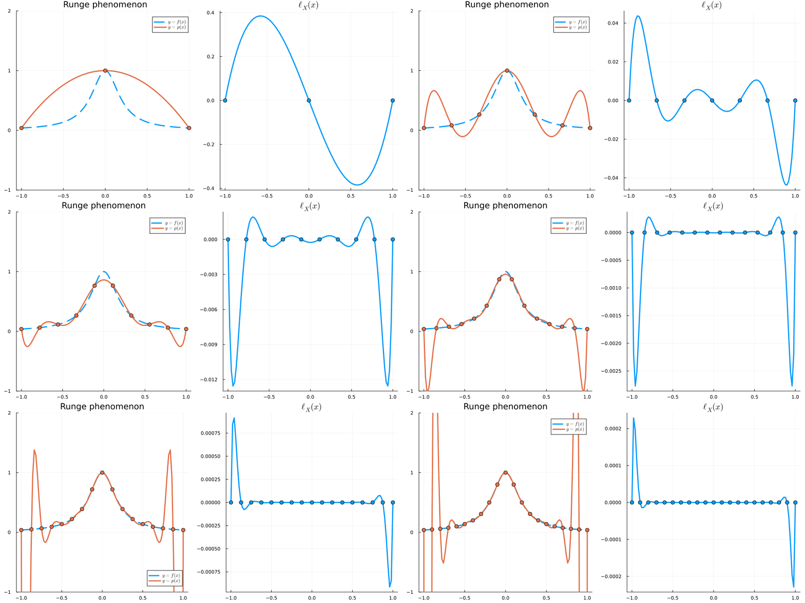
Chebyshev nodes (of the second kind) on \([-1,1]\) are given by
\[ \begin{align} X = \Big\{ \cos \frac{j\pi}{n} \Big\}_{j=0}^n \end{align} \tag{6.2}\]
n = 10
θ = range(0, π, length=n+1)
px, py = cos.(θ), sin.(θ)

t = range(0, π, length=400)
plt = plot(cos.(t), sin.(t);  lw = 2, color = :black, label = "",
        aspect_ratio = :equal, legend = :topright,
        xlims = (-1.15, 1.15), ylims = (-0.15, 1.15), grid = false)
plot!(plt, [-1, 1], [0, 0], color = :black, lw = 1, label = "")

for j in eachindex(px)
    plot!(plt, [px[j], px[j]], [py[j], 0];
        ls = :dash, color = :gray, label = "")
end

scatter!(plt, px, py;
    ms = 5, color = :blue, label = "Equispaced on semi-circle")

scatter!(plt, px, zeros(length(px));
    ms = 5, color = :red, label = "Chebyshev nodes")
N = 25

err = zeros(N)
egrid = -1:.01:1

anim = @animate for n ∈ 2:N
    x = @. cos( π*(0:n)/n )
    y = @. f₃( x )

    p = fit(ChebyshevT, x, y)

    plt1 = plot(f₃, -1, 1;
            label=L"y = f(x)", lw = 3, linestyle = :dash, title = "Chebyshev Interpolation")
    plot!(plt1, p, -1, 1;
            label=L"y = p(x)", lw = 3 )
    scatter!(plt1, [x], [y];
            primary = false, ylims=(-.1,1.1), markersize = 5)

    ℓ = fromroots( x )
    plt2 = plot(ℓ, -1, 1;
            title=L"\ell_X(x)", legend = false, lw = 3)
    scatter!(plt2, [x], [zeros(n)];
            primary = false, markersize = 5)

    hline!(plt2, [2.0^(1-n), -2.0^(1-n)]; linestyle=:dash )
    plot( plt1, plt2; size=(1000, 500))
    err[n] = maximum( @. abs( p(egrid) - f₃(egrid) ) )
end

gif(anim, "../images/Chebyshev.gif", fps = 1)
┌ Info: Saved animation to c:\Users\jack6\Projects\Math5485-Fall-2026\images\Chebyshev.gif
└ @ Plots C:\Users\jack6\.julia\packages\Plots\GIume\src\animation.jl:156
scatter( 2:N, err[2:end] ;
    yaxis= :log, title="Absolute error", legend=false, lw = 3)
plot!(2:N, @. 2*((1+sqrt(26))/5)^(- (2:N) );
    linestyle = :dash )
For \(x \in [-1,1]\), we have
\[\begin{align} |\ell_X(x)| &\leq \frac{e}{2\sqrt{n}} \left( \frac2e \right)^n &\text{for Equispaced nodes } X = \Big\{ \frac{2j-n}{n} \Big\}_{j=0}^n \nonumber\\ % |\ell_X(x)| &\leq 2^{1-n} &\text{for Chebyshev nodes } X = \Big\{ \cos \frac{j\pi}{n} \Big\}_{j=0}^n \nonumber \end{align}\]
Example 6.3 Possible presentation topic: Numerical study of the convergence behaviour of Chebyshev interpolation. e.g.:
N = 25

err = zeros(N)
egrid = -1:.01:1

anim = @animate for n ∈ 2:N
    x = @. cos( π*(0:n)/n )
    y = @. f₄( x )

    p = fit(ChebyshevT, x, y)

    plt1 = plot(f₄, -1, 1, label=L"y = f(x)", lw = 3, linestyle = :dash, title = "Chebyshev interpolation: hat function")
    plot!(plt1, p, -1, 1, label=L"y = p(x)", lw = 3 )
    scatter!(plt1, [x], [y], primary = false, ylims=(-.1,1.1), markersize = 5)

    err[n] = maximum( @. abs( p(egrid) - f₄(egrid) ) )

end

gif(anim, "../images/Hat.gif", fps = 1)
┌ Info: Saved animation to c:\Users\jack6\Projects\Math5485-Fall-2026\images\Hat.gif
└ @ Plots C:\Users\jack6\.julia\packages\Plots\GIume\src\animation.jl:156
scatter( 2:N, err[2:end];
    xaxis= :log, yaxis= :log, title="Absolute error", legend=false, lw = 3)
plot!( 2:N, (2:N).^(-1);
    linestyle=:dash )
Exercise 6.4 Consider \(f(x) = e^{-x}\) on \([-1,1]\).
Find a Lagrange interpolating polynomial \(p\) of \(f\) on \(\{ -1, 0 , 1\}\),
Write down an error estimate for approximating \(f\) with \(p\) on \([-1,1]\).
Exercise 6.5 (Growth of the equispaced node polynomial) (\(\star\) more difficult)
Let \(X = \{x_0 < \cdots < x_n\}\) be \(n+1\) equispaced nodes on \([-1,1]\), i.e. \(x_j = -1 + jh\) with \(h = 2/n\), and let \(\ell_X(x) = (x-x_0)(x-x_1)\cdots(x-x_n)\) be the node polynomial.
Fix \(x \in [x_k, x_{k+1}]\) for some \(0 \leq k \leq n-1\). By bounding \(|x - x_j|\) for \(j < k\) and \(j > k+1\) and using \(|x-x_k|\,|x-x_{k+1}| \leq h^2/4\), show that
\[ |\ell_X(x)| \leq \frac{h^{n+1}}{4} (k+1)!\,(n-k)!, \]
and deduce that \(\max_{x\in[-1,1]} |\ell_X(x)| \leq \dfrac{n!}{4} h^{n+1}\).
Use Stirling’s formula, \(n! \sim \sqrt{2\pi n}\,(n/e)^n\), to show that there is a constant \(C > 0\), independent of \(n\), such that
\[ \max_{x\in[-1,1]} |\ell_X(x)| \leq C\, \frac{(2/e)^n}{\sqrt n} \qquad \text{for all } n. \]
By evaluating \(\ell_X\) at the point \(x^* = x_0 + h/2\), show that there is a constant \(c > 0\), independent of \(n\), such that
\[ \max_{x\in[-1,1]} |\ell_X(x)| \geq c\, \frac{(2/e)^n}{n} \qquad \text{for all } n. \]
Note that \(2/e \approx 0.736\): parts 2 and 3 together show that \(\max\limits_{x\in[-1,1]} |\ell_X(x)|\) decays exponentially, but at a rate no better than \((2/e)^n\).
Exercise 6.6 (A convergence threshold for Runge’s example) (\(\star\) more difficult)
Fix \(\alpha > 0\) and let \(f(x) = \dfrac{1}{1+\alpha x^2}\), as in Example 6.2 (with \(\alpha=25\)).
Using the geometric series \(f(x) = \sum_{k=0}^\infty (-\alpha)^k x^{2k}\) for \(|x| < 1/\sqrt\alpha\), show that
\[\begin{align} f^{(2k)}(0) &= (2k)!\,(-\alpha)^k, \nonumber\\ f^{(2k+1)}(0) &= 0. \nonumber \end{align}\]
Using partial fractions (the poles of \(f\) are at \(x = \pm i/\sqrt\alpha\)), show more generally that
\[ \max_{x \in [-1,1]} |f^{(n)}(x)| = n!\, \alpha^{n/2}, \]
with the maximum attained at \(x=0\).
Combine part 2 with Exercise 6.5 and Theorem 6.2 to show that, for \(X\) the equispaced nodes on \([-1,1]\),
\[ |f(x) - I_Xf(x)| \leq C\sqrt\alpha \, \frac{1}{\sqrt n} \left( \frac{2\sqrt\alpha}{e} \right)^n, \]
and deduce that this bound converges to \(0\) whenever \(\alpha < \frac{e^2}{4} \approx 1.847\).
It turns out that we have convergence for all \(\alpha < \alpha_{\rm c} \approx 3.621\) Trefethen (2019), Epperson (1987).
Next week, we will see that for Chebyshev nodes, the node polynomial instead satisfies \(|\ell_X(x)| \leq 2^{1-n}\) and so
\[ |f(x) - I_Xf(x)| \leq 2\sqrt\alpha \left( \frac{\sqrt\alpha}{2} \right)^n, \]
which converges to \(0\) whenever \(\alpha < 4\). (A sharper argument, using that \(f\) is analytic throughout a neighbourhood of \([-1,1]\) in \(\mathbb C\) rather than just bounding derivatives along the real axis shows that Chebyshev interpolation converges for all \(\alpha > 0\).)