📢 Updates

Lecture 9: Hermite interpolation available Assignment 3 available Lecture 8 online Lecture 7 online Schedule now available in "Admin" Problem class exercises now online Lecture 6 online Quiz 1 solutions online Lectures 2-3 exercises have solutions! Lecture 1 exercises have solutions!

3  Conditioning & stability

Lecture 3: Conditioning and stability and the start of Chapter 2: Solving nonlinear equations in 1d

Warning

These lecture notes are mainly a record of what we discussed in class. They should not be used as a replacement for attending lectures or reading books. Please let me know if you find any errors or have any questions about the material.

TipHypothesis

You can use the Hypothesis commenting system available on the right side panel (you can login with your U/Google account). This allows you annotate the notes (private) and leave comments or reply to other people’s comments (public).

Note

I encourage you to download the lecture notes and play around with the Julia code.

Download (.ipynb) Ask a Question ChimeIn (opens in a new tab)

Note

This lecture is based on Chapter 1 of [Fundamentals of Numerical Computation by Driscoll, Braun] which is avaliable online (opens in a new tab)

3.1 Recap

ChimeIn: floating point numbers, round off error, …

Exercise 3.1

Let \(\epsilon\) be the machine precision. Is \((1 + \epsilon/2) - 1 = 1 + (\epsilon/2-1)\) in Float64?

ϵ = eps( Float64 )
(1.0 + ϵ/2) - 1.0 == 1.0 + (ϵ/2 - 1.0)

false

This is false, since \(1 + \epsilon\) is the smallest float larger than \(1\), Julia has to round or truncate \(1 + \epsilon/2\):

1 + ϵ/2

1.0

Therefore, \((1 + \epsilon/2) -1 = 0\). On the other hand \(\epsilon/2 - 1\) is a float and so \(1 + (\epsilon/2 - 1)\) is not equal to \(0\).

Exercise 3.2

Let \(X\) be an array containing \(10^{16}, -10^{16}\), and \(N\) copies of \(1\). What is the sum of all the entries of the array \(X\)? Does it depend on the order of summation? What about in Float64? Why?

using Random

N = 10^2
X = vcat( [1e16, -1e16], fill(1., N) )

for _ ∈ 1:10 
    shuffle!(X)
    s = 0. 
    for x ∈ X
        s += x 
    end
    println(s)
end 

72.0
32.0
92.0
25.0
44.0
94.0
77.0
96.0
55.0
26.0

This happens because \(2^{53} \leq 10^{16} < 2^{54}\) and so the spacing between floats in this interval is \(2^{n-k} = 2^{53-52} = 2\) (in Float64, the binary precision is \(k=52\)). As a result \(10^{16} + 1\) is not a float; Julia rounds this to \(10^{16}\):

1e16 + 1

1.0e16

WarningSubtractive cancellation

When adding or subtracting numbers so that the result is much smaller in magnitude. For example, we know \(x = -1.0000000000000000000147\) to \(23\) significant digits but \(x + 1 = -1.47 \times 10^{-20}\) to only \(3\) significant digits.

This concept can be illustrated using (relative) condition number:

3.2 Conditioning

Suppose we are interested in a quantity \(f(x)\) for \(x\in \mathbb R\). In practice, we can only store \(\widetilde{x} := \mathrm{fl}(x)\) in a computer (recall that \(\widetilde{x} = x(1 + \epsilon)\) for some \(|\epsilon|\leq \frac12 \epsilon_{\mathrm{mach}}\)). Then the ratio of the relative error in the output to the relative error in the input in the limit as the precision goes to zero is known as the (relative) condition number \(\kappa_f(x)\):

Definition 3.1 (Relative condition number) \[\begin{align} \kappa_f(x) := \lim_{\epsilon\to0}\left| \frac {f(x) - f(x + \epsilon x)} {\epsilon f(x)} \right| \nonumber % \end{align}\]

That is, the (relative) condition number is approximately the constant of proportionality between the relative error in the output and the relative error of the input:

\[\begin{align} \left|\frac {f(x) - f(\widetilde{x})} {f(x)} \right| \approx \kappa_f(x) \left|\frac {x - \widetilde{x}} {x} \right| % = \kappa_f(x) |\epsilon|. \nonumber \end{align}\]

Example 3.1 The condition number of \(f(x) = x + 1\) is \(\kappa_f(x) = \left|\frac{x}{x+1}\right|\). This blows up when \(x\approx -1\) which explains subtractive cancellation that we mentioned above.

Definition 3.2 If the condition number is large, we say the problem is ill-conditioned or the problem is badly conditioned

Notice that

\[\begin{align} \kappa_f(x) &= \lim_{\epsilon\to0}\left| \frac {f(x) - f(x + \epsilon x)} {\epsilon f(x)} \right| \nonumber\\ % &= \lim_{\epsilon\to0}\left| \frac {f(x) - f(x + \epsilon x)} {\epsilon x} \right| \left| \frac{x}{f(x)} \right| \nonumber\\ % &= \left| \frac{x f'(x)}{f(x)} \right| \end{align}\]

Exercise

Exercise 2.8

Example 3.2 (Polynomial roots as a function of monomial basis coefficients) The polynomial

\[\begin{align} a \xi^2 + b \xi + c = 0 \end{align}\]

has roots \(\xi_1,\xi_2\). Fix \(b,c\) and consider \(\xi_1 = \xi_1(a)\). What is \(\kappa_{\xi_1}(a)\)?

Warning

For higher-order polynomials, representing functions in the standard monomial basis (\(\{1, x, x^2, \dots\}\)) is usually a bad idea. Monomial bases are ill-conditioned; tiny perturbations in the coefficients can drastically change the behaviour of the polynomial and shift the roots significantly. To maintain numerical stability, it’s a better idea to use to an orthogonal basis like Chebyshev polynomials (see later in the semester).

Potential presentation topics include: Wilkinson’s Polynomial, conditioning of Vandermonde matrices, understand and explain this, this, ….

Poor conditioning is a problem with the problem! On the other hand, if we see a large error in the result, the problem might be with the solution! That is, the algorithm can also introduce errors. When the error can not be explained by an ill-conditioned problem, we will say the algorithm is unstable.

3.3 Stability: An Example

Consider \(\xi^2 - (10^n + 10^{-n})\xi + 1 = 0\). The roots of this equation are \(\xi_1 := 10^{-n}\) and \(\xi_2 := 10^n\). These roots are well separated so we expect the problem of finding the roots to be well-conditioned. We show below that the quadratic formula is unstable.

The quadratic formula in floating point arithmetic gives:

n = 8;
a, b, c = 1, -(10.0^n + 10.0^(-n)), 1;
ξ1, ξ2 = ( -b - sqrt( b^2 - 4*a*c) )/(2*a), ( -b + sqrt( b^2 - 4*a*c) )/(2*a);

@show ( ξ1, ξ2 ) ;

(ξ1, ξ2) = (1.4901161193847656e-8, 1.0e8)

The error in approximating the first root is quite big!

println( "relative errors = (", abs( ξ1 - 10.0^(-n) )/10.0^(-n) , ", ", abs( ξ2 - 10.0^n )/10.0^n, ")" )

relative errors = (0.49011611938476557, 0.0)

But why?

-b

1.0000000000000001e8

sqrt( b^2 - 4 * a * c )

9.999999999999999e7

-b - sqrt( b^2 - 4*a*c)

2.9802322387695312e-8

The error is coming from Subtractive Cancellation! The quadratic formula is thus ill-conditioned. Alternatively we could compute \(\xi_1\) from \(\xi_2\):

ξ1 = (c/a)/ξ2

1.0e-8

Which is exact in Float64.

Another way of computing \(\xi_1\) is to rationalise the numerator:

\[\begin{align} \xi_1 &= \frac{ -b - \sqrt{ b^2 - 4ac } }{2a} \\ % &= \frac{ -b - \sqrt{ b^2 - 4ac } }{2a} \times \frac{ -b + \sqrt{ b^2 - 4ac } }{-b + \sqrt{ b^2 - 4ac } } \nonumber\\ % &= \frac { b^2 - ( b^2 - 4ac ) } {2a( -b + \sqrt{ b^2 - 4ac } )} \\ % &= \frac { 2c } { -b + \sqrt{ b^2 - 4ac } } \end{align}\]

Using this formula, we get

ξ1 = 2*c / ( -b + sqrt(b^2 - 4*a*c) )

1.0e-8

Which is again exact in Float64

3.4 FNC Exercises

We then looked at questions 1.4.1 and 1.4.2 from [Fundamentals of Numerical Computation by Driscoll, Braun]

Exercise 3.3

Exercise 1.4.1 from Driscoll and Braun (2017), [Fundamentals of Numerical Computation by Driscoll, Braun]

f = x -> (1 - cos(x) )/sin(x)
g = x -> 2*sin(x/2)^2/sin(x)

(f(1e-6), g(1e-6))

(5.000444502912538e-7, 5.000000000000416e-7)

Since \(1 - \cos x = 2 \sin^2 \frac{x}{2}\), the formulas \(f(x) = \frac{1 - \cos x}{\sin x}\) and \(g(x) = \frac{2 \sin^2(x/2)}{\sin x}\) are mathematically identical (both equal \(\tan \frac{x}{2}\)).

In floating point, however, they are different for small \(x\). For \(x = 10^{-6}\) (see the code above):

• \(f(10^{-6}) \approx 5.000444 \times 10^{-7}\), with relative error \(\approx 9 \times 10^{-5}\) (only about \(4\) correct significant digits),
• \(g(10^{-6}) \approx 5.000000000000416 \times 10^{-7}\), which is correct to machine precision (relative error \(\approx 10^{-16}\)).

The problem itself is well-conditioned: with \(F(x) = \tan\frac{x}{2}\), we have \(\kappa_F(x) = \left|\frac{x F'(x)}{F(x)}\right| = \frac{x}{\sin x} \approx 1\) for small \(x\). The large error in \(f\) is therefore due to the algorithm: \(\cos(10^{-6}) \approx 1 - 5 \times 10^{-13}\), so computing \(1 - \cos x\) subtracts two nearly equal numbers (subtractive cancellation) and loses about \(12\) significant digits. The formula \(g\) involves no such subtraction, and so is stable.

Exercise 3.4

Exercise 1.4.2 from Driscoll and Braun (2017), [Fundamentals of Numerical Computation by Driscoll, Braun]

x = @. 10.0^(-(1:11));
f = @. (exp(x) - 1)/x;

p=1;
for n ∈ 1:8
    p = @. p + x^n/( factorial(n+1) );
end 

abs.(f-p) ./ x

11-element Vector{Float64}:
    1.1102230246251565e-14
    1.0880185641326532e-12
    4.285460875053104e-11
    4.32542890393961e-9
    9.701794922989393e-7
    3.798317216308078e-5
    0.005663214341922184
    1.1077470940534795
   82.24037095772019
  826.9037099495335
 8273.537099867668

# upper bound on the error between f and p as functions on x
err = @. (1/factorial(10)) * (x^9/(1-x))

11-element Vector{Float64}:
 3.061924358220656e-16
 2.7835675983824175e-25
 2.7584904128114e-34
 2.7560075231509052e-43
 2.7557594799933906e-52
 2.755734678133266e-61
 2.7557321979718108e-70
 2.755731949955909e-79
 2.755731925154322e-88
 2.7557319226741635e-97
 2.755731922426145e-106

Using the Taylor expansion of \(e^x\), we have

\[\begin{align} f(x) = \frac{e^x - 1}{x} = \sum_{n=0}^\infty \frac{x^n}{(n+1)!}, \qquad p(x) := \sum_{n=0}^{8} \frac{x^n}{(n+1)!}. \nonumber \end{align}\]

For \(0 < x < 1\), the truncation error satisfies

\[\begin{align} |f(x) - p(x)| = \sum_{n = 9}^\infty \frac{x^n}{(n+1)!} \leq \frac{1}{10!} \sum_{n=9}^\infty x^n = \frac{x^9}{10!\,(1-x)}, \nonumber \end{align}\]

which is less than \(3.1 \times 10^{-16}\) for \(x \leq 0.1\) (see the second code cell above). Since \(f(x) \geq 1\), the polynomial \(p\) is accurate to machine precision for all \(x \in (0, 0.1]\).

On the other hand, the formula \(\frac{e^x - 1}{x}\) suffers from subtractive cancellation for small \(x\) (\(e^x \approx 1\)): its relative error grows roughly like \(\epsilon_{\rm mach}/x\), from \(\approx 10^{-14}\) at \(x = 10^{-2}\) to \(\approx 10^{-8}\) at \(x = 10^{-8}\). The differences \(|f - p|\) computed above are therefore almost entirely the error of the naive formula, not the truncation error of \(p\). (Julia’s expm1 avoids this problem: expm1(x)/x is accurate for all small \(x\).)

3.5 Chapter 2. Solving nonlinear equations in 1d

Note

This chapter will be mainly based on Chapter 1 of Süli and Mayers (2003).

Definition 3.3 We say \(\xi\) is a root (or a zero) of \(f: [a,b] \to \mathbb R\) if \(f(\xi) = 0\).

• Simple functions can be solved explicitly e.g. \(ax^2 + bx + c = 0\) (also true for degree \(3,4\))
  
• \(x^5 - 4x - 2 = 0\) - no closed formula for roots of this equation

p = Polynomial([-2, -4, 0, 0, 0, 1]) 
@show p;

plot(p, legend=false)
plot!( real( filter( isreal, roots(p) ) ), zeros(3), seriestype=:scatter )

p = Polynomial(-2 - 4*x + x^5)

• Need numerical methods to get the roots!
• Aim: for \(f: [a,b] \to \mathbb R\), solve \(f(\xi) = 0\) for \(\xi \in \mathbb R\),
• Also, can find \(\xi\) such that \(f(\xi) = y\) (by considering \(x \mapsto f(x) - y\)) or stationary points (by considering \(f = F'\)),
• Simple examples with no solution, e.g. \(f(x) = x^2 + 1\)

Theorem 3.1 (Intermediate value theorem) Suppose that \(f : [a,b] \to \mathbb R\) is continuous and \(f(a) < y < f(b)\) or \(f(b) < y < f(a)\). Then, there exists a \(c\in [a,b]\) such that \(f(c) = y\).

This result, implies the following useful theorem for determining whether a function has a root:

Theorem 3.2 (Change of sign) If \(f\) is continuous on \([a,b]\) and \(f(a) f(b) \leq 0\) then there exists \(\xi \in [a,b]\) with \(f(\xi) = 0\).

Proof. If \(f(a) f(b) = 0\) then either \(a\) or \(b\) is a root. We can therefore suppose that \(f(a) f(b) < 0\) and so either \(f(a) < 0 < f(b)\) or \(f(b) < 0 < f(a)\). Since \(f\) is continuous, we can apply the intermediate value theorem on \(f\) to conclude there exists a root \(c \in [a,b]\).

Warning

The converse to this theorem is untrue. i.e. there exists \(f\) with a real root in \([a,b]\) but with \(f(a)f(b) > 0\).

Exercise 3.5

Let \(f(x) = e^x - 2x - 1\). Apply change of sign theorem to \(f\) to conclude there exists \(\xi \in [1,2]\) such that \(f(\xi) = 0\).

The function \(f(x) = e^x - 2x - 1\) is continuous with \(f(1) = e - 3 \approx -0.28 < 0\) and \(f(2) = e^2 - 5 \approx 2.39 > 0\). Therefore, \(f(1) f(2) < 0\) and, by the change of sign theorem, there exists \(\xi \in [1,2]\) with \(f(\xi) = 0\).

f = x -> exp(x) - 2*x - 1;
@show ( f(1), f(2) )

plot( f, 1, 2; label = L"y = f(x)" )
plot!( x->0; label = L"y = 0", linestyle=:dot )

(f(1), f(2)) = (-0.2817181715409549, 2.3890560989306504)

Definition 3.4 We say \(\xi\) is a fixed point of \(g: [a,b] \to \mathbb R\) if \(g(\xi) = \xi\).

• We can rewrite \(f(\xi) = 0\) as a fixed point problem \(g(\xi) = \xi\) (for example, we could define \(g(x) := x \pm f(x)\)).

The change of sign theorem can be applied here:

Theorem 3.3 (Brouwer’s fixed point theorem) Suppose \(g : [a,b]\to\mathbb R\) is continuous with \(g(x) \in [a,b]\) for all \(x \in [a,b]\). Then, there exists \(\xi\in [a,b]\) with \(g(\xi) = \xi\).

Proof. We can apply the change of sign theorem to \(f(x) := g(x) - x\). Indeed, because \(g(a), g(b) \in [a,b]\), we have \(f(a) = g(a) - a \geq 0\) and \(f(b) = g(b) - b \leq 0\) and thus \(f\) is continuous with \(f(a) f(b) \leq 0\). All roots \(\xi\in[a,b]\) of \(f\) are fixed points of \(g\).

Exercise 3.6

Let’s return to Exercise 3.5. You showed that \(f(x) = e^x - 2x - 1\) has a root \(\xi \in [1,2]\).

Show that \(f(x) = 0\) can be solved by instead considering the fixed point problems \(g(x) = x\) or \(h(x) = x\) where

\[ \begin{align} g(x) &= \log( 2x + 1 ), \\ h(x) &= \frac{e^x - 1}{2}. \end{align} \tag{3.1}\]

Show that Brouwer’s fixed point theorem applies to \(g\) but not \(h\) on \([1,2]\).

For \(x \in [1,2]\) we have \(2x + 1 > 0\), and \(\log\) is one-to-one, so

\[\begin{align} g(x) = x &\iff \log(2x+1) = x \nonumber\\ &\iff 2x + 1 = e^x \nonumber\\ &\iff f(x) = 0, \nonumber \end{align}\]

and

\[\begin{align} h(x) = x &\iff \frac{e^x - 1}{2} = x \nonumber\\ &\iff e^x - 2x - 1 = 0 \nonumber\\ &\iff f(x) = 0. \nonumber \end{align}\]

That is, the roots of \(f\) are exactly the fixed points of \(g\) and of \(h\).

\(g\): \(g\) is continuous and increasing on \([1,2]\), with \(g(1) = \log 3 \approx 1.10\) and \(g(2) = \log 5 \approx 1.61\). So, for all \(x \in [1,2]\),

\[\begin{align} 1 < g(1) \leq g(x) \leq g(2) < 2. \nonumber \end{align}\]

Therefore \(g : [1,2] \to [1,2]\) and Brouwer’s fixed point theorem gives a fixed point \(\xi = g(\xi) \in [1,2]\).

\(h\): \(h(1) = \frac{e - 1}{2} \approx 0.86 < 1\) (and \(h(2) = \frac{e^2 - 1}{2} \approx 3.19 > 2\)), so \(h\) does not map \([1,2]\) into \([1,2]\) and Brouwer’s fixed point theorem does not apply. (Of course, \(h\) still has the fixed point \(\xi \in [1,2]\) found above: the theorem just cannot be used to show it.)

g = x -> log( 2*x + 1 );    
h = x -> (exp(x) - 1)/2;
id = x -> x;

@show (g(1), g(2));
@show (h(1), h(2));

plot( [g, h, id], 1, 2, label=[L"g" L"h" L"x"])
hline!(  [1, 2]; linestyle=:dot, color=:black, primary=false )

(g(1), g(2)) = (1.0986122886681098, 1.6094379124341003)
(h(1), h(2)) = (0.8591409142295225, 3.194528049465325)

TipTO-DO

• Assignment 1: Due today!
• Exercises throughout the notes,
• Extra research: Research a time when real world problems have occurred when floating point numbers have not been implemented properly (add to the discussion on canvas)
• Extra reading: myths of polynomial interpolation
• (Sign-up to office hours if you like)

3.6 Extra exercises

Exercise 3.7 (Lambert W function)

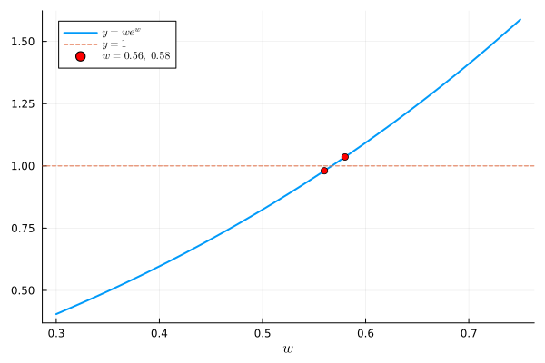
Assignment 1, Fall 2025, [30 pts]. Prove that, for \(x \geq 0\), there exists a unique \(W(x) \geq 0\) for which \(W(x) e^{W(x)} = x\). Show that \(\Omega := W(1)\) satisfies \(0.56 < \Omega < 0.58\).

Intermediate value theorem is useful!

The function \(F(w) := w e^w\) is continuous on \([0, \infty)\) with \(F(0) = 0\) and \(F(w) \to \infty\) as \(w \to \infty\). Therefore, for \(x \geq 0\), there exists \(w_x \geq 0\) with \(F(0) \leq x \leq F(w_x)\) and, by the intermediate value theorem, there exists \(W \in [0, w_x]\) with \(F(W) = x\). Moreover, \(F'(w) = (1 + w) e^w > 0\), so \(F\) is strictly increasing on \([0,\infty)\): if \(W' < W < W''\) then \(F(W') < x < F(W'')\). Hence \(W(x) := W\) is the unique solution in \([0,\infty)\) of \(W e^W = x\).

Finally, \(F(0.56) = 0.56\, e^{0.56} \approx 0.980 < 1\) and \(F(0.58) = 0.58\, e^{0.58} \approx 1.035 > 1\), and so (again since \(F\) is continuous and strictly increasing) \(\Omega = W(1) \in (0.56, 0.58)\). In the plot below, \(\Omega\) is where the curve \(y = w e^w\) crosses the line \(y = 1\):

using Plots, LaTeXStrings
F = w -> w * exp(w)

plot( F, 0.3, 0.75; label = L"y = w e^w", xlabel = L"w", lw = 2, legend = :topleft )
hline!( [1]; label = L"y = 1", linestyle = :dash )
scatter!( [0.56, 0.58], F.([0.56, 0.58]); label = L"w = 0.56,\ 0.58", color = :red )

Exercise 3.8

Assignment 2, Fall 2025, [10 pts]. For fixed \(f\), define

\[\begin{align} g(x) &= f(x - a), \\ h(x) &= b f(x), \\ j(x) &= f(c x), \end{align}\]

1. What is \(\kappa_g(x)\)?
2. Write \(\kappa_{h}(x)\) in terms of \(\kappa_f\),
3. Write \(\kappa_{j}(x)\) in terms of \(\kappa_f\),
4. What is \(\kappa_f(x)\) when \(f(x) = e^{-x^2}\)?

Recall that \(\kappa_f(x) = \left| \frac{x f'(x)}{f(x)} \right|\).

1. \(g'(x) = f'(x - a)\) and so \(\kappa_g(x) = \left| \frac{x f'(x-a)}{f(x-a)} \right| = \left| \frac{x}{x - a} \right| \kappa_f(x - a)\).
2. \(h'(x) = b f'(x)\) and so \(\kappa_h(x) = \left| \frac{x\, b f'(x)}{b f(x)} \right| = \kappa_f(x)\) (for \(b \not= 0\)): scaling the output doesn’t change the conditioning.
3. \(j'(x) = c f'(cx)\) and so \(\kappa_j(x) = \left| \frac{x\, c f'(cx)}{f(cx)} \right| = \kappa_f(cx)\). (Common mistakes: \(|c| \kappa_f(cx)\), \(\frac{1}{|c|}\kappa_f(x)\), or \(\frac{1}{|c|}\kappa_f(cx)\).)
4. \(f'(x) = -2x e^{-x^2}\) and so \(\kappa_f(x) = \left| \frac{x \cdot (-2x) e^{-x^2}}{e^{-x^2}} \right| = 2x^2\).

Exercise 3.9

Assignment 2, Fall 2025, [25 pts]. Consider the differential equation (initial value problem)

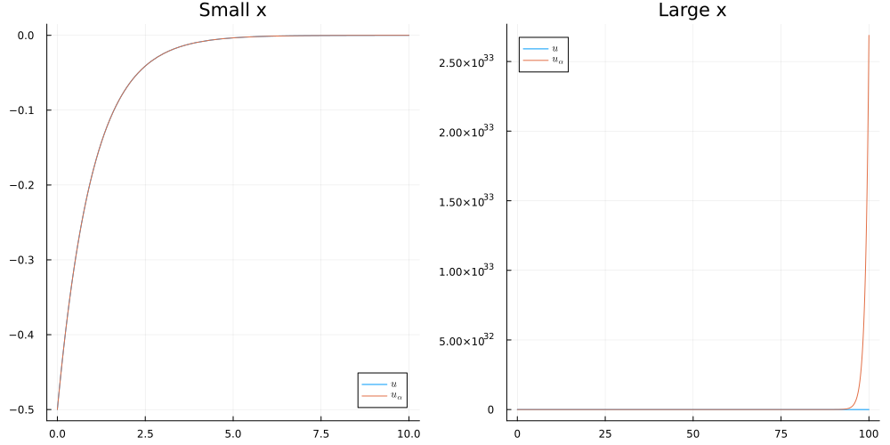
\[ \begin{align} \begin{split} u'(x) &= u(x) +e^{-x} \nonumber \\ u(0) &= -\frac12 . \end{split} \end{align} \tag{3.2}\]

1. Show that \(u(x) = -\frac12 e^{-x}\) solves (3.2).

Now we perturb the initial data, by considering

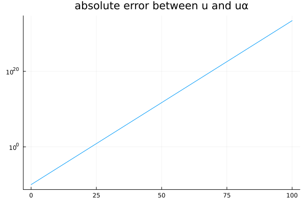
\[ \begin{align} \begin{split} u'(x) &= u(x) +e^{-x} \nonumber \\ u(0) &= \alpha \end{split} \end{align} \tag{3.3}\]

for \(\alpha := \epsilon - \frac12\).

2. Show that \(u_{\alpha}(x) = (\alpha + \frac12) e^x -\frac12 e^{-x}\) solves (3.3).
3. Plot the functions \(u\) and \(u_{\alpha}\) and comment on the difference between the solutions for large \(x\).
4. Let \(f( \alpha ) = u_\alpha( 100 )\). What is the condition number \(\kappa_f( \alpha )\)?
5. Explain what happens for \(\alpha \approx -\frac12\). Link your observations to your answer for question 3.

1. \(u'(x) = \frac12 e^{-x} = -\frac12 e^{-x} + e^{-x} = u(x) + e^{-x}\) and \(u(0) = -\frac12\).

2. \(u_\alpha'(x) = (\alpha + \frac12) e^x + \frac12 e^{-x} = u_\alpha(x) + e^{-x}\) and \(u_\alpha(0) = (\alpha + \frac12) - \frac12 = \alpha\).

3. The difference between the two solutions is \(u_\alpha(x) - u(x) = (\alpha + \frac12) e^{x} = \epsilon e^x\). Here are \(u\) and \(u_\alpha\) for \(\epsilon = 10^{-10}\):

α = 1e-10 - 1/2;

u = x -> -exp(-x)/2;
uα = x -> (α + 1/2)*exp(x) + u(x);

plt1 = plot([u, uα], 0, 10, label=[L"u" L"u_\alpha"], title="Small x")
plt2 = plot([u, uα], 0, 100, label=[L"u" L"u_\alpha"], title="Large x")

plot( plt1, plt2, size=(1000,500))

For small \(x\) (left) the two solutions are indistinguishable: \(u_\alpha(x) \approx u(x)\). For large \(x\) (right) they are completely different: \(u(x) = -\frac12 e^{-x}\) decays to \(0\), whereas \(u_\alpha(x) \approx \epsilon e^x\) grows exponentially. For example, \(u(20) \approx -10^{-9}\) but \(u_\alpha(20) \approx 0.05\), and \(u(30) \approx -5 \times 10^{-14}\) but \(u_\alpha(30) \approx 1069\).

The difference is easiest to see on a logarithmic scale:

err = x -> abs( u(x) - uα(x) ) 

plot( err, 0, 100 , yaxis=:log, legend = false, title="absolute error between u and uα" )

On a logarithmic \(y\)-axis, the error \(|u(x) - u_\alpha(x)| = \epsilon e^x\) is a straight line with slope \(1\) (in natural-log units): a perturbation of size \(\epsilon = 10^{-10}\) in the initial condition grows by a factor \(e\) for every unit increase in \(x\), and is about \(3 \times 10^{33}\) at \(x = 100\).

4. \(f(\alpha) = u_\alpha(100) = (\alpha + \frac12) e^{100} - \frac12 e^{-100}\) and \(f'(\alpha) = e^{100}\), so \[\begin{align} \kappa_f(\alpha) = \left| \frac{\alpha f'(\alpha)}{f(\alpha)} \right| = \left| \frac{\alpha e^{100}}{(\alpha + \frac12) e^{100} - \frac12 e^{-100}} \right|. \nonumber \end{align}\]

5. As \(\alpha \to -\frac12\), \(\kappa_f(\alpha) \to \left| \frac{-\frac12 e^{100}}{-\frac12 e^{-100}} \right| = e^{200} \approx 7 \times 10^{86}\): the problem is extremely ill-conditioned. A tiny relative change in the initial condition (e.g. storing \(-\frac12 + \epsilon\) in floating point) leads to a huge relative change in \(u(100)\), which is exactly what the plots in part 3 show.

   For example, with \(\epsilon = 10^{-10}\) as in the plots: the relative change in the input is \(\left|\frac{\epsilon}{-1/2}\right| = 2 \times 10^{-10}\), while \(u(100) \approx -1.9 \times 10^{-44}\) and \(u_\alpha(100) \approx 2.7 \times 10^{33}\), a relative change of about \(1.4 \times 10^{77}\) in the output. Their ratio is \(\approx 7.2 \times 10^{86} \approx e^{200} \approx \kappa_f(\alpha)\), as predicted.

Exercise 3.10

Assignment 2, Fall 2025, [10 pts]. Let \(p_{\alpha}(x) = \alpha x^n + \sum_{j=0}^{n-1} a_{j} x^j\) be a polynomial of degree \(n\) and let \(r(\alpha)\) be a root of \(p_{\alpha}\). What is the condition number \(\kappa_r(\alpha)\)?

Since \(p_\alpha(r(\alpha)) = 0\) for all \(\alpha\), differentiating with respect to \(\alpha\) gives

\[\begin{align} r(\alpha)^n + p_\alpha'\big(r(\alpha)\big)\, r'(\alpha) = 0 \qquad \text{and so} \qquad r'(\alpha) = - \frac{r(\alpha)^n}{p_\alpha'\big(r(\alpha)\big)} \nonumber \end{align}\]

(assuming \(r(\alpha)\) is a simple root, so that \(p_\alpha'(r(\alpha)) \not= 0\)). Therefore,

\[\begin{align} \kappa_r(\alpha) = \left| \frac{\alpha\, r'(\alpha)}{r(\alpha)} \right| = \left| \frac{\alpha\, r(\alpha)^{n-1}}{p_\alpha'\big(r(\alpha)\big)} \right|. \nonumber \end{align}\]

In particular, the root is ill-conditioned when \(p_\alpha'(r(\alpha))\) is small, i.e. when \(r(\alpha)\) is close to a repeated root.

Driscoll, Tobin A., and Richard J. Braun. 2017. Fundamentals of Numerical Computation. Society for Industrial; Applied Mathematics. https://doi.org/10.1137/1.9781611975086.

Süli, Endre, and David F. Mayers. 2003. An Introduction to Numerical Analysis. Cambridge, England: Cambridge University Press. https://doi.org/10.1017/CBO9780511801181.